Some background
I was long fascinated by the visual depictions of bird sounds shown in the Golden Guide to the Birds of North America. These graphics, called sonagrams or spectrograms, display the frequency content of the sounds (usually songs) as a function of time. I acquired a few interesting books on bird sounds and found out that people had been visually depicting bird songs for many years, either using musical staff notation (“Born to Sing”, Charles Harstone, Indiana University Press, 1973) or by using simple line drawings of pitch versus time (“A Guide to Bird Songs,” Aretas A. Saunders, Doubleday & Company, 1935). Unfortunately, neither of these methods adequately displays the impressive harmonic content of a typical bird song. A major breakthrough was the commercial appearance of the Sonagraph by the Kay Electric Company in 1951. This electronic device used a sensitive receiver and appropriate audio filters to drive a pen recorder and make plots of the spectral content of audio signals as a function of time. These are the plots that appear in the Golden Guide and other books such as “Bird Sounds,” Gerhard A. Thielke, University of Michigan Press, 1976, and the Dover series of books and tapes by Donald J. Borror (“Birds Song and Behavior”, “Songs of Eastern Birds”, “Common Bird Songs.”)
My system
By 1991 I had done a lot of work on time-domain radar, and recognized that it should be possible to create sonagrams from digitized signals using a short-time Fourier transform. These days anyone can create beautiful sonagrams on a smart phone, but in 1991 it looked to be a fun challenge. Sound cards for the IBM PC (such as Sound Blaster) had just recently become available, but were still quite expensive. I didn’t want to kluge my own A/D converter, so I opted to buy a COVOX Voice Master, which was designed for rudimentary voice recognition. It could also record speech to a file using an 8-bit A/D converter, and I could access the raw data from the files. I wrote some BASIC code to process the data on my 8 MHz PC-XT clone, and print sonagrams on my el-cheapo dot matrix printer. I tested it on some pre-recorded bird songs and was able to calibrate the plots pretty well.
With the software working, I decided to try my hand at recording some sounds from nature and making my own sonagrams. I bought a $50 Radio Shack portable cassette recorder, but found that the built-in microphone did not do a very good job of picking up distant bird songs. So I opted to add a little $50 amplified microphone from Edmund Scientific, bringing the total cost of my system up to $250 — not exactly a professional audio system! There was a lot of wind and background noise, but I was able to eliminate a lot using very simple techniques like frequency windowing and thresholding. The results are really quite satisfying for such a primitive approach.
My sonagrams
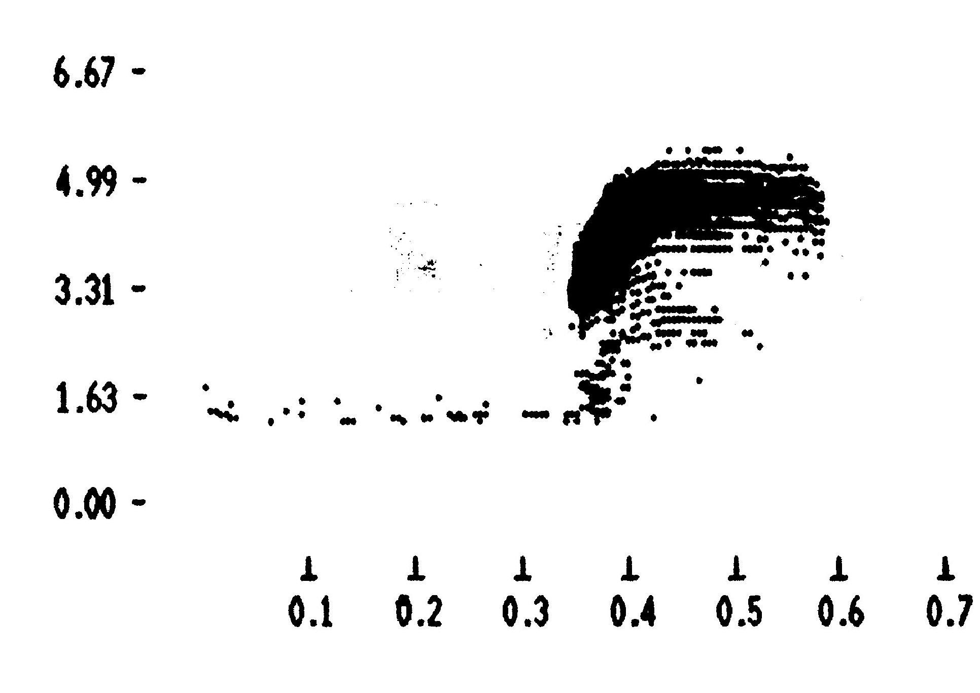
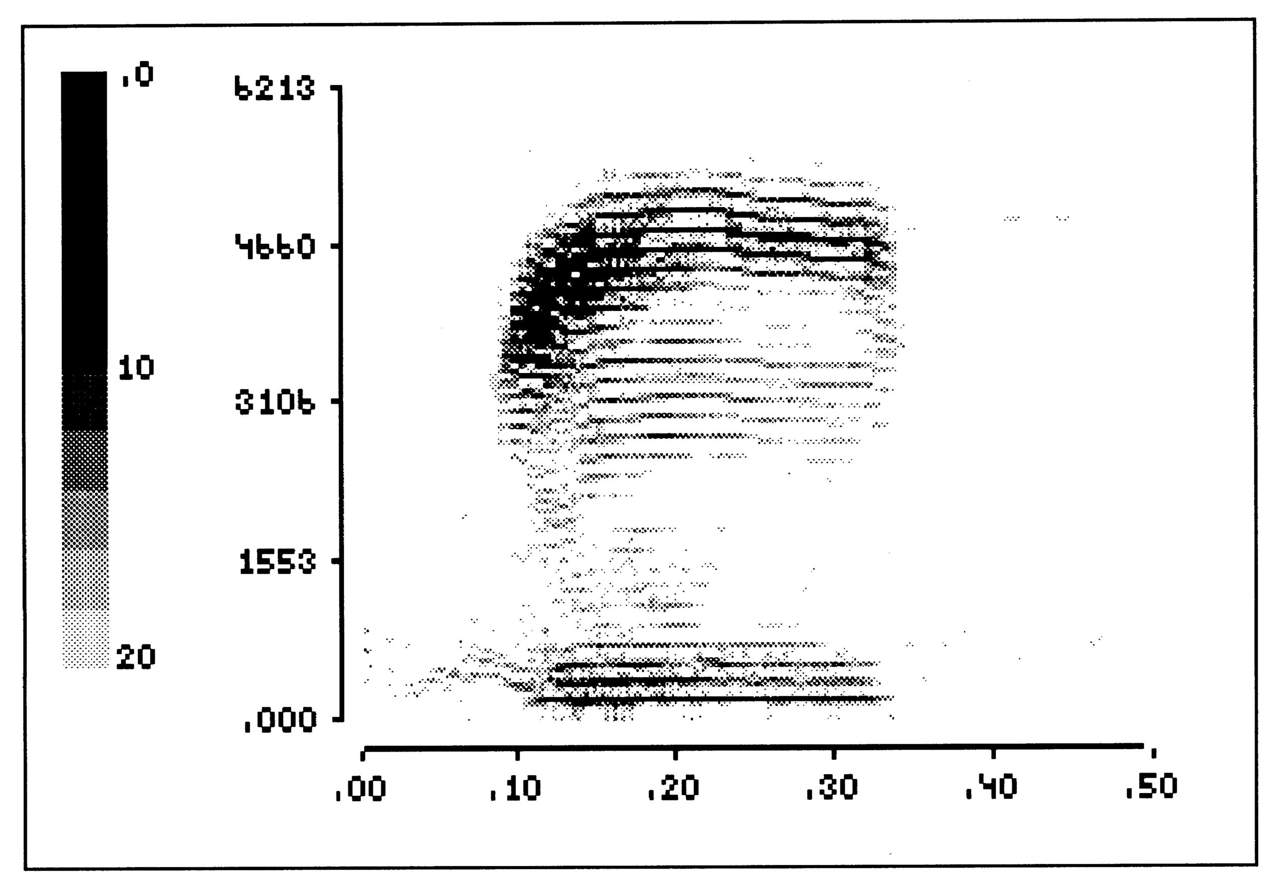
When you look at the sonagrams linked below, you’ll see several different styles of plots. The first version of my BASIC code used a simple amplitude threshold – if the signal strength at a certain frequency was above a set level, a black dot was plotted; otherwise not. This produced simple plots that look a lot like those in the Golden Guide. For instance, the “bzeep” call of the American woodcock is shown in the plot at the top of the page. You can tell that there is a lot of harmonic content, but it’s difficult to resolve the individual harmonics. In 1992 I upgraded to a newer dot matrix printer, and I also got a more powerful 386SX computer. I rewrote the BASIC code a couple of more times, and eventually started plotting variations in amplitudes using shading; this produced the plot shown here. What a difference! It’s possible to count 28 distinct harmonics within the measurement band of the recording and digitizing systems. This is quite amazing!
And then…
I went on to record a large number of birds, frogs, insects, and other sounds from nature. I made sonagrams and stored everything on 5.25 inch floppy disks; sadly, these were long ago lost. Recently, I discovered a group of the printouts, which I have scanned and posted below. The rest, including the ones from insects, are lost forever. That’s almost the end of the story, except that I showed some of the plots to one of my graduate students, Jack Ross, who suggested we apply my code to our radar data. I was skeptical at first, but eventually our research group got some very useful results and published this short journal paper. If you’re into signal processing, you might recognize the plots as being similar to the time-frequency analysis provided using wavelets. That’s because the short-time FFT is akin to a very simple wavelet transform.
For the nerdy
Here’s the BASIC code I used to create the final version of the sonagram plots. Tools like Matlab were in their infancy, and agonizingly expensive, so it made sense to program my own plotting routines. Note that the code for computing the fast Fourier transform (FFT) is missing. I used a standard 2^N point FFT routine I had written in BASIC back in grad school. (I wrote the FFT code for a numerical analysis class on my very first computer — an Ohio Scientific Challenger IIP, which I got in 1979. This computer had a whopping 4k of RAM, and Microsoft Basic — Bill Gates’ first commercial product — in ROM.)
The sonagrams
Frogs
- Green frogs chorusing: sonagram with summary
- Wood frog: sonagram with summary
Birds
- American crow caw: sonagram with summary
- American goldfinch:
- song 1: sonagram sonagram with summary
- song 2: sonagram sonagram with summary
- American robin:
- laugh: sonagram sonagram with summary
- song: sonagram sonagram with summary
- American woodcock:
- breaking into flight: sonagram with summary
- descending flight: sonagram with summary
- bzeep call: sonagram sonagram with summary
- bzeep call: sonagram
- multiple bzeep calls: sonagram with summary
- Black-capped chickadee: sonagram with summary
- Blue jay:
- scream: sonagram sonagram with summary
- squeaky gate: sonagram sonagram with summary
- Carolina wren song: sonagram with summary
- Chipping sparrow call: sonagram sonagram with summary
- Common flicker call: sonagram sonagram with summary
- Common grackle: sonagram with summary
- Common yellowthroat:
- song1: sonagram sonagram and summary
- song2: sonagram with summary
- Dark-eyed junco song: sonagram sonagram with summary
- Eastern meadowlark song: sonagram with summary
- Eastern phoebe: sonagram sonagram with summary
- Eastern wood pewee:
- first two notes: sonagram sonagram with summary
- last two notes: sonagram sonagram with summary
- Gray catbird:
- calls: sonagram with summary
- more calls: sonagram with summary
- mew: sonagram with summary
- song:
- part 1: sonagram with summary
- part 2: sonagram with summary
- part 3: sonagram with summary
- Great crested flycatcher song: sonagram sonagram with summary
- Great horned owl hoot: sonagram sonagram with summary
- Hermit thrush song:
- part 1: sonagram with summary
- part 2: sonagram with summary
- part 3: sonagram with summary
- House wren song: sonagram sonagram with summary
- Indigo bunting song: sonagram sonagram with summary
- Marsh wren song:
- part 1: sonagram with summary
- part 2: sonagram with summary
- part 3: sonagram with summary
- Meadowlark song: sonagram sonagram and summary
- Northern oriole song: sonagram with summary
- Northern cardinal:
- Ascending call:
- part 1: sonagram with summary
- part 2: sonagram with summary
- part 3: sonagram with summary
- Descending call:
- part 1: sonagram with summary
- part 2: sonagram with summary
- Ascending call:
- Northern oriole:
- song 1: sonagram
- song 2: sonagram sonagram with summary
- song 3: sonagram sonagram with summary
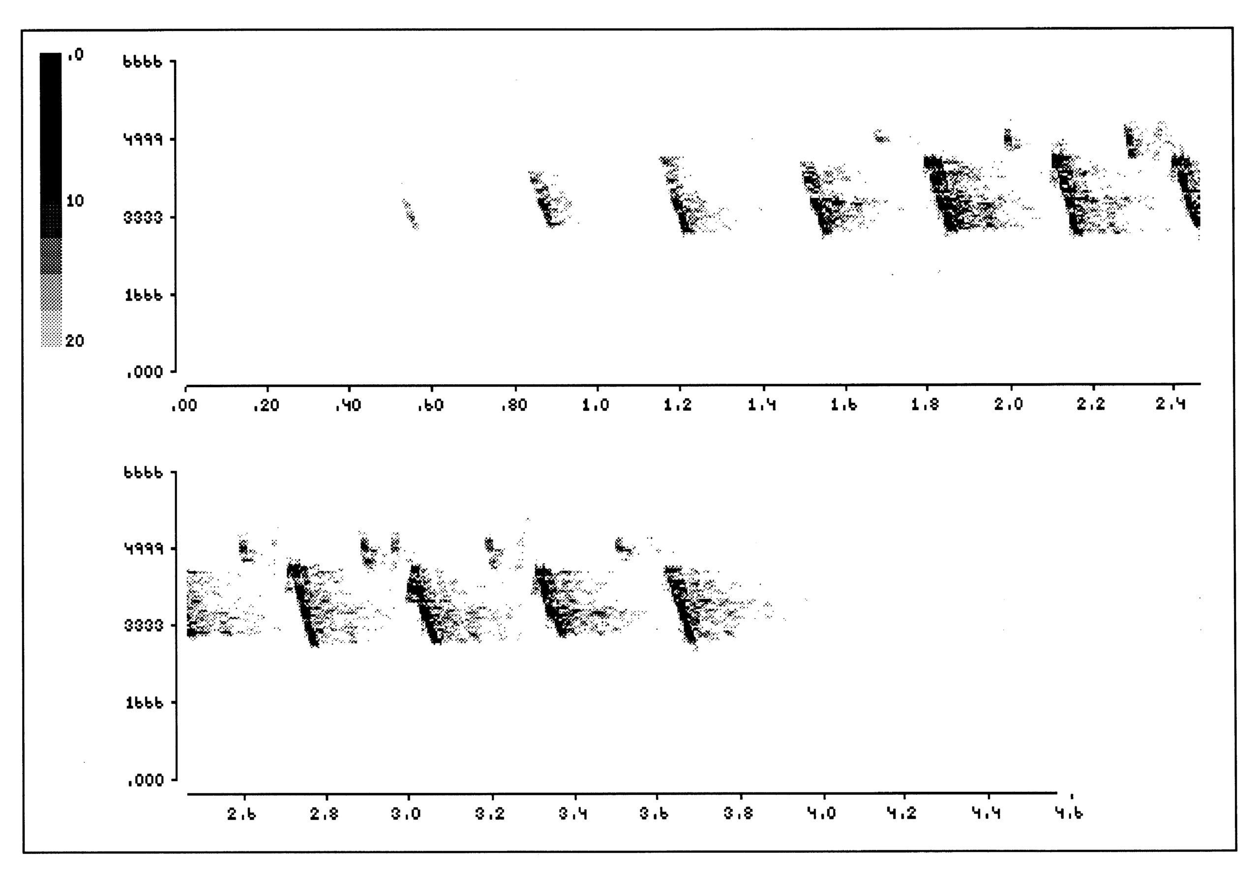
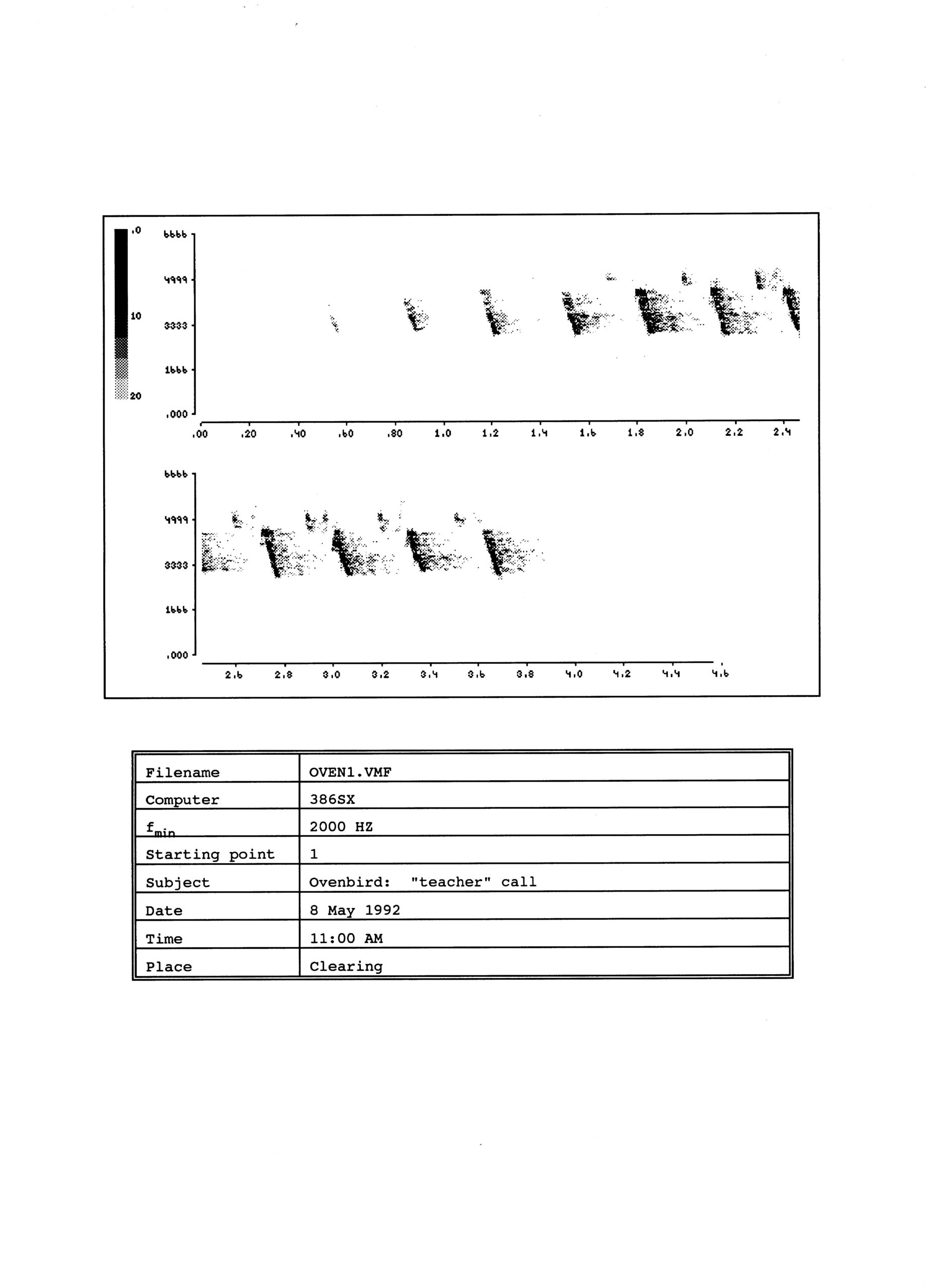
- Ovenbird teacher call: sonagram sonagram with summary
- Pileated woodpecker:
- call: sonagram sonagram with summary
- drumming: sonagram sonagram with summary
- Purple finch song: sonagram with summary
- Red-bellied woodpecker call: sonagram with summary
- Red-eyed vireo song: sonagram with summary
- Redwing blackbird song: sonagram with summary
- Rooster crowing: sonagram sonagram with summary
- Rose-breasted grosbeak:
- song 1: sonagram sonagram with summary
- song 2: sonagram sonagram with summary
- song 3: sonagram sonagram with summary
- Scarlet tanager chip-burr call:
- part 1: sonagram with summary
- part 1: sonagram with summary
- Song sparrow:
- song 1: sonagram sonagram with summary
- song 2: sonagram with summary
- Veery:
- calls:
- calls 1: sonagram with summary
- calls 2: sonagram with summary
- calls and song:
- calls and song plot type 1: sonagram sonagram with summary
- calls and song plot type 2: sonagram with summary
- calls:
- White-throated sparrow:
- 2-note song: sonagram sonagram with summary
- old sam peabody song: sonagram sonagram with summary
- Yellow-bellied sapsucker: sonagram with summary